Examples
This Jupyter
Notebook
aims at showing the properties of the expandLHS module.
>>> import numpy as np
>>> import matplotlib.pyplot as plt
>>> from scipy.stats.qmc import LatinHypercube
>>> # the following import ensure to load the latest version of the module
>>> # the user should install the module and then import it as usual
>>> from importlib.machinery import SourceFileLoader
>>> expandLHS = SourceFileLoader("expandLHS", "../expandLHS/expandLHS.py").load_module()
>>> from expandLHS import ExpandLHS
>>> import plotter
Matplotlib is building the font cache; this may take a moment.
Expand a Latin Hypercube
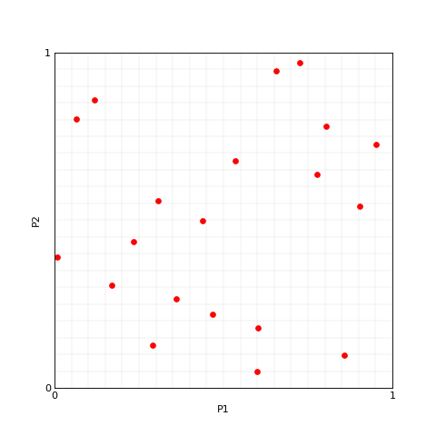
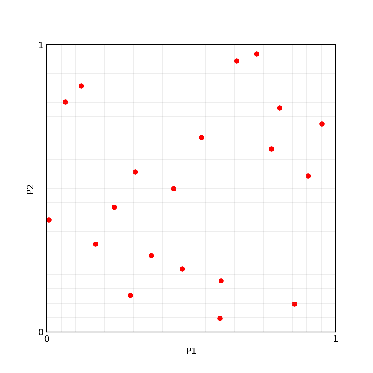
Let’s start sampling a random Latin Hypercube as implemented in Scipy.stats.qmc.LatinHypercube.
>>> N = 20 # number of samples
>>> P = 2 # number of dimensions
>>>
>>> lhs_sampler = LatinHypercube(P)
>>> lhs_set = lhs_sampler.random(N)
>>>
>>> plotter.plot(lhs_set, M=0, x_label='P1', y_label='P2');

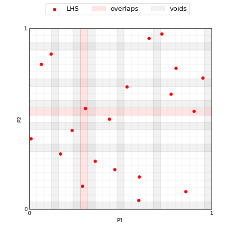
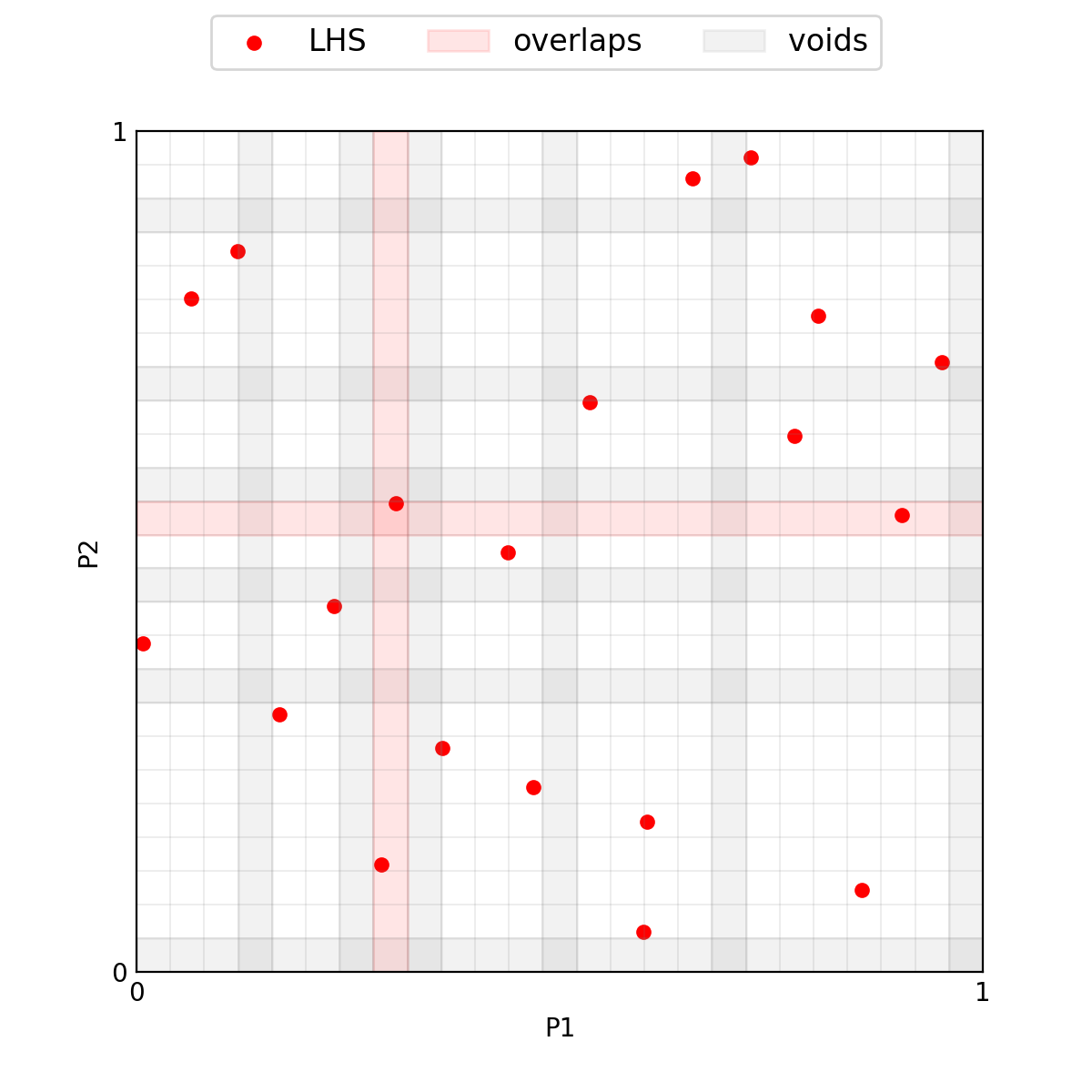
Now the aim is to add new samples without modifying the ones we already sampled. This procedure may cause two samples to fall in the same interval, even if they do not overlap in the initial set.
As a first step we need to resize the binning of the intervals, we can
see the effect of this by running ExpandLHS.regridding explicitly.
The method ExpandLHS.count_samples allows to compute the number of
samples in each interval for each dimension, this can be used to detect
eventual overlaps. It is not necessary to call these two methods
explicitly to expand an LHS, their outputs are used here for explanatory
reason.
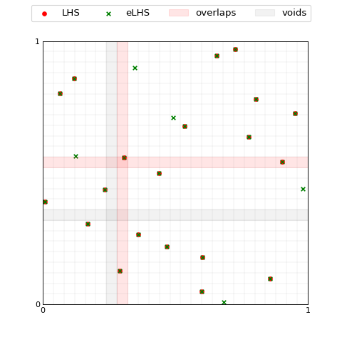
>>> M = 5 # number of samples to add
>>>
>>> eLHS = ExpandLHS(lhs_set)
>>> voids = eLHS._regridding(M)
>>> overlaps = eLHS._count_samples(M)
>>>
>>> #the plot function internally compute both voids and overlaps
>>> plotter.plot(lhs_set, M=M, labels='LHS', voids=voids, overlaps=overlaps, x_label='P1', y_label='P2');

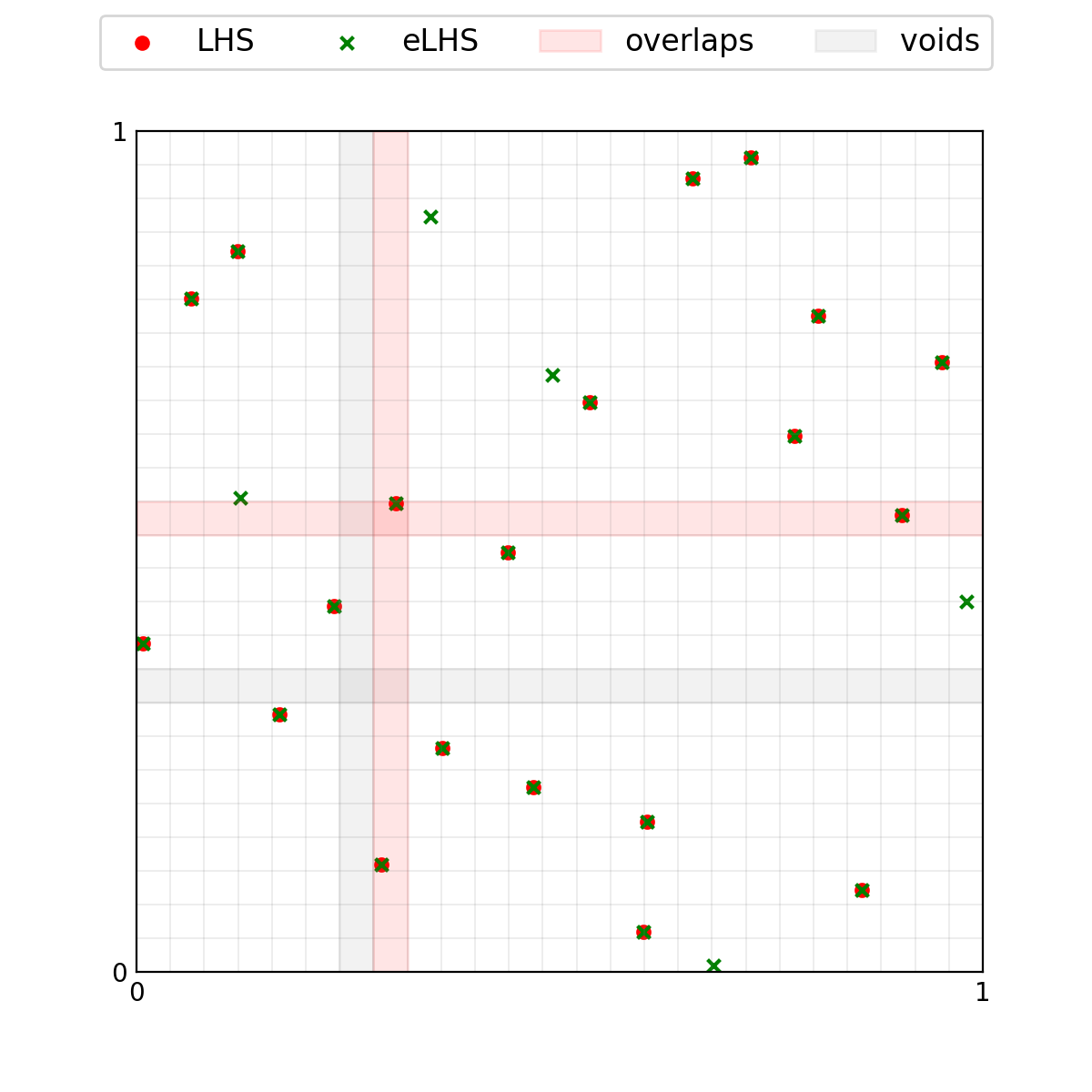
The class call ExpandLHS.__call__ performs the entire expansion
process, thus it regrids the hypercube accounting for the new points and
performs the sampling.
>>> lhs_set_expanded = eLHS(M)
>>> voids = eLHS._regridding(0, samples=lhs_set_expanded) #recompute voids on the expanded set
>>>
>>> plotter.plot([lhs_set, lhs_set_expanded], M=0, labels=['LHS', 'eLHS'], \
...     colors=['red', 'green'], markers=['o', 'x'], sizes=[25, 25], \
...     index = 1, voids=voids, overlaps=overlaps);
Degree of an expansion
The regridding of the space may cause some overlaps and voids, which imply that the new set is not a Latin Hypercube anymore.
We define a metric to measure the degree-of-LHS of a samples set. This
estimate is performed with the method ExpandLHS.degree. A perfect
Latin Hypercube has always a degree of 1.
>>> degree = eLHS.degree(M)
>>> print(f'LHS degree = {degree:.3f}')
LHS degree = 0.920
Using the method ExpandLHS.optimal_expansion it is possible to
compute the degree-of-LHS for different expansion sizes in a given
interval.
>>> expansions = eLHS.optimal_expansion((4, 9), verbose=True)
>>> print(f'List of expansions sorted by the corresponding degree:\n')
>>> for expansion in expansions:
...     print(f'({expansion[0]}, {expansion[1]:.4f})')
List of expansions sorted by the corresponding degree:
(0, 1.0000) (9, 0.9483) (8, 0.9464) (7, 0.9259) (5, 0.9200) (4, 0.9167) (6, 0.8654)
Optimized expansion
Scipy’s implementation of Latin Hypercube sampling allows to optimize the sample set using the centered discrepancy. A lower value for this metric corresponds to a better space-filling of the hypercube.
>>> from scipy.stats.qmc import discrepancy, geometric_discrepancy
>>>
>>> N = 50
>>> P = 6
>>> M = 42
>>>
>>> lhs_sampler = LatinHypercube(P)
>>> lhs_set = lhs_sampler.random(N)
>>> lhs_sampler_opt = LatinHypercube(P, optimization='random-cd')
>>> lhs_set_opt = lhs_sampler_opt.random(N)
>>>
>>> print(f'''
>>> Discrepancy of LHS without optimization: {discrepancy(lhs_set):.4f} \n
>>> Discrepancy of LHS with optimization: {discrepancy(lhs_set_opt):.4f}''')
Discrepancy of LHS without optimization: 0.0131
Discrepancy of LHS with optimization: 0.0058
ExpandLHS.__call__ is it possible to ask for an
optimized expansion with the keyword optimize=, where the
available metrics are: - discrepancy
(Scipy.stats.qmc.discrepancy)>>> eLHS = ExpandLHS(lhs_set_opt)
>>> lhs_set_expanded = eLHS(M)
>>> lhs_set_expanded_opt = eLHS(M, optimize='discrepancy')
>>>
>>> print(f'''
>>> Discrepancy of eLHS without optimization: {discrepancy(lhs_set_expanded):.4f} \n
>>> Discrepancy of eLHS with optimization: {discrepancy(lhs_set_expanded_opt):.4f}''')
Discrepancy of eLHS without optimization: 0.0055
Discrepancy of eLHS with optimization: 0.0049
>>> eLHS = ExpandLHS(lhs_set_opt)
>>> lhs_set_expanded = eLHS(M)
>>> lhs_set_expanded_opt = eLHS(M, optimize='geometric_discrepancy')
>>>
>>> print(f'''
>>> Discrepancy of eLHS without optimization: {geometric_discrepancy(lhs_set_expanded):.4f} \n
>>> Discrepancy of eLHS with optimization: {geometric_discrepancy(lhs_set_expanded_opt):.4f}''')
Discrepancy of eLHS without optimization: 0.2382
Discrepancy of eLHS with optimization: 0.3104